Data

Data from simulations performed by McStasScript is returned as McStasData objects. This section will explore what these contain and how one can manipulate them. First a small instrument is written that will supply data to investigate.

Example instrument

The instrument will consist of a source, a powder sample and some monitors that will record data.

Show code cell source

Hide code cell source

import mcstasscript as ms

instrument = ms.McStas_instr("data_example")

source = instrument.add_component("source", "Source_simple")
source.set_parameters(xwidth=0.05, yheight=0.03, dlambda=0.1,
                      dist=5, focus_xw=0.015, focus_yh=0.03)
source.lambda0 = instrument.add_parameter("wavelength", value=1.2)

sample = instrument.add_component("sample", "PowderN")
sample.set_parameters(radius=source.focus_xw, yheight=source.focus_yh,
                      reflections='"Na2Ca3Al2F14.laz"', barns=0)
sample.set_AT(source.dist, RELATIVE=source)

Example monitors

Here three monitors are defined, a 2D PSD monitor, a 1D banana monitor and an event monitor. Monitor_nD is used for the last two, where the option string describes the geometry and what is to be recorded.

banana = instrument.add_component("banana", "Monitor_nD", RELATIVE=sample)
banana.set_parameters(xwidth=1.5, yheight=0.4, restore_neutron=1, filename='"banana.dat"')
banana.options = '"theta limits=[5 175] bins=250, banana"'

event = instrument.add_component("events", "Monitor_nD")
event.set_AT(0.1, RELATIVE=sample)
event.set_parameters(xwidth=0.1, yheight=0.1, restore_neutron=1, filename='"events.dat"')
event.options = '"list all auto, x y z vx vy vz t"'

mon = instrument.add_component("PSD", "PSD_monitor")
mon.set_AT(0.1, RELATIVE=sample)
mon.set_parameters(nx=100, ny=100, filename='"psd.dat"',
                   xwidth=3*sample.radius, yheight=2*sample.yheight, restore_neutron=1)

Generating data

The simulation is executed using the backengine method with a low number of neutrons. The data is returned by the backengine method, but will contain None if the simulation failed.

instrument.settings(ncount=1E5, output_path="data_example")
data = instrument.backengine()

INFO: Using directory: "/home/runner/work/McStasScript/McStasScript/docs/source/user_guide/data_example"
INFO: Regenerating c-file: data_example.c
CFLAGS= @NCRYSTALFLAGS@
          
WARNING:
 The parameter format of sample is initialized 
 using a static {,,,} vector.
  -> Such static vectors support literal numbers ONLY.
  -> Any vector use of variables or defines must happen via a 
     DECLARE/INITIALIZE pointer.


-----------------------------------------------------------

Generating single GPU kernel or single CPU section layout: 

-----------------------------------------------------------

Generating GPU/CPU -DFUNNEL layout:

-----------------------------------------------------------
INFO: Recompiling: ./data_example.out
lto-wrapper: warning: using serial compilation of 3 LTRANS jobs
lto-wrapper: note: see the '-flto' option documentation for more information
/home/runner/micromamba/envs/mcstasscript-docs/bin/x86_64-conda-linux-gnu-ld: /tmp/ccyMrKqq.ltrans1.ltrans.o: in function `read_line_data.constprop.0':
/home/runner/work/McStasScript/McStasScript/docs/source/user_guide/./data_example.c:10259:(.text.read_line_data.constprop.0+0xea): warning: the use of `tmpnam' is dangerous, better use `mkstemp'
INFO: ===
Opening input file '/home/runner/micromamba/envs/mcstasscript-docs/share/mcstas/resources/data/Na2Ca3Al2F14.laz' (Table_Read_Offset)
Table from file 'Na2Ca3Al2F14.laz' (block 1) is 841 x 18 (x=1:20), constant step. interpolation: linear
  '# TITLE *-Na2Ca3Al2F14-[I213] Courbion, G.;Ferey, G.[1988] Standard NAC cal ...'
PowderN: sample: Reading 841 rows from Na2Ca3Al2F14.laz
PowderN: sample: Powder file probably of type Lazy Pulver (laz)
WARNING: but F2 unit is set to barns=0 (fm^2). Intensity might be 100 times too low.
PowderN: sample: Read 841 reflections from file 'Na2Ca3Al2F14.laz'
PowderN: sample: Vc=1079.1 [Angs] sigma_abs=11.7856 [barn] sigma_inc=13.6704 [barn] reflections=Na2Ca3Al2F14.laz
*** TRACE end *** 
Detector: banana_I=2.63842e-07 banana_ERR=6.71234e-09 banana_N=10701 "banana.dat"
Events:   "events_dat_list.p.x.y.z.vx.vy.vz.t"
Detector: PSD_I=4.96614e-05 PSD_ERR=5.02109e-07 PSD_N=10410 "psd.dat"
PowderN: sample: Info: you may highly improve the computation efficiency by using
    SPLIT 504 COMPONENT sample=PowderN(...)
  in the instrument description data_example.instr.
INFO: Placing instr file copy data_example.instr in dataset /home/runner/work/McStasScript/McStasScript/docs/source/user_guide/data_example
INFO: Placing generated c-code copy data_example.c in dataset /home/runner/work/McStasScript/McStasScript/docs/source/user_guide/data_example

print(data)

[
McStasData: banana type: 1D  I:2.63842e-07 E:6.71234e-09 N:10701.0, 
McStasDataEvent: events with 12442 events. Variables: p x y z vx vy vz t, 
McStasData: PSD type: 2D  I:4.96614e-05 E:5.02109e-07 N:10410.0]

McStasData objects

The data retrieved from the instrument object is in the form of a list that contains McStasDataBinned and McStasDataEvent objects. McStasScript contains a function called name_search which can be used to select a certain element of such a data list. It will match the component name first and if no match is found it will check for match with the filename. Here name_search is used to retrieve the PSD McStasDataBinned object.

PSD = ms.name_search("PSD", data)
banana = ms.name_search("banana", data)
events = ms.name_search("events", data)

Accessing metadata

Both McStasDataBinned and McStasDataEvent object carries relevant metadata in a metadata attribute. Using the python print function this object can display basic information on the contained data.

print(PSD.metadata)
print(banana.metadata)
print(events.metadata)

metadata object
component_name: PSD
filename: psd.dat
2D data of dimension (100, 100)
  [-2.25: 2.25] X position [cm]
  [-3.0: 3.0] Y position [cm]
 Signal per bin
Instrument parameters: 
 wavelength = 1.2

metadata object
component_name: banana
filename: banana.dat
1D data of length 250
  [5.0: 175.0] Longitude [deg]
 Intensity [n/s/bin]
Instrument parameters: 
 wavelength = 1.2

metadata object
component_name: events
filename: events_dat_list.p.x.y.z.vx.vy.vz.t
2D data of dimension (8, 12442)
  [1.0: 12442.0] List of neutron events
  [1.0: 8.0] p x y z vx vy vz t
 Signal per bin
Instrument parameters: 
 wavelength = 1.2

The metadata object has attributes which can be accessed as well. The info attribute is a dict with the raw metadata read from the file.

• component_name

• dimension

• filename

• limits

• parameters

• info

PSD.metadata.info

{'Date': 'Fri Jul 24 18:50:36 2026 (1784919036)',
 'type': 'array_2d(100, 100)',
 'Source': 'data_example (data_example.instr)',
 'component': 'PSD',
 'position': '0 0 5.1',
 'title': 'PSD monitor',
 'Ncount': '100000',
 'filename': 'psd.dat',
 'statistics': 'X0=-0.00842687; dX=0.443828; Y0=0.00291527; dY=0.877722;',
 'signal': 'Min=0; Max=7.59544e-08; Mean=4.96614e-09;',
 'values': '4.96614e-05 5.02109e-07 10410',
 'xvar': 'X',
 'yvar': 'Y',
 'xlabel': 'X position [cm]',
 'ylabel': 'Y position [cm]',
 'zvar': 'I',
 'zlabel': 'Signal per bin',
 'xylimits': '-2.25 2.25 -3 3',
 'variables': 'I I_err N',
 'Parameters': {'wavelength': 1.2}}

The total intensity, error or ncount is kept in the values are often of interest, so these are given their own attributes: total_I, total_E and total_N

print(PSD.metadata.total_I)
print(PSD.metadata.total_E)
print(PSD.metadata.total_N)

4.96614e-05
5.02109e-07
10410.0

Accessing the data

McStasData objects stores the data as Numpy arrays, these can be accessed as attributes.

• Intensity: Holds the intensity, sum of all ray weights

• Error: Error on intensity

• Ncount: Number of rays that reached

print("Intensity")
print(PSD.Intensity)

print("Error")
print(PSD.Error)

print("Ncount")
print(PSD.Ncount)

Intensity
[[0.00000000e+00 0.00000000e+00 0.00000000e+00 ... 0.00000000e+00
  0.00000000e+00 1.90717902e-10]
 [0.00000000e+00 0.00000000e+00 0.00000000e+00 ... 0.00000000e+00
  0.00000000e+00 1.87576210e-10]
 [0.00000000e+00 0.00000000e+00 0.00000000e+00 ... 0.00000000e+00
  0.00000000e+00 0.00000000e+00]
 ...
 [0.00000000e+00 0.00000000e+00 0.00000000e+00 ... 0.00000000e+00
  0.00000000e+00 0.00000000e+00]
 [0.00000000e+00 0.00000000e+00 0.00000000e+00 ... 0.00000000e+00
  0.00000000e+00 0.00000000e+00]
 [0.00000000e+00 0.00000000e+00 0.00000000e+00 ... 0.00000000e+00
  0.00000000e+00 9.22040689e-12]]
Error
[[0.00000000e+00 0.00000000e+00 0.00000000e+00 ... 0.00000000e+00
  0.00000000e+00 1.90717902e-10]
 [0.00000000e+00 0.00000000e+00 0.00000000e+00 ... 0.00000000e+00
  0.00000000e+00 1.87576210e-10]
 [0.00000000e+00 0.00000000e+00 0.00000000e+00 ... 0.00000000e+00
  0.00000000e+00 0.00000000e+00]
 ...
 [0.00000000e+00 0.00000000e+00 0.00000000e+00 ... 0.00000000e+00
  0.00000000e+00 0.00000000e+00]
 [0.00000000e+00 0.00000000e+00 0.00000000e+00 ... 0.00000000e+00
  0.00000000e+00 0.00000000e+00]
 [0.00000000e+00 0.00000000e+00 0.00000000e+00 ... 0.00000000e+00
  0.00000000e+00 9.22040689e-12]]
Ncount
[[0. 0. 0. ... 0. 0. 1.]
 [0. 0. 0. ... 0. 0. 1.]
 [0. 0. 0. ... 0. 0. 0.]
 ...
 [0. 0. 0. ... 0. 0. 0.]
 [0. 0. 0. ... 0. 0. 0.]
 [0. 0. 0. ... 0. 0. 1.]]

The original path to the data is also contained within the McStasData object and can be returned with get_data_location.

PSD.get_data_location()

'/home/runner/work/McStasScript/McStasScript/docs/source/user_guide/data_example'

Event data

McStasDataEvent objecst stores event data, and for this reason does not have Error or Ncount. The event information is contained in a 2D Numpy array in the Intensity and Events attributes.

print(events)

McStasDataEvent: events with 12442 events. Variables: p x y z vx vy vz t

print("Events", events.Events)

Events [[ 5.10138308e-09  7.64480428e-03 -5.16950445e-03 ... -1.11530500e+01
   3.08604474e+03  1.65260080e-03]
 [ 5.08311737e-09 -4.53435570e-03  1.22565770e-02 ...  1.52443760e+01
   3.32157612e+03  1.53541566e-03]
 [ 5.09151791e-09  5.38774762e-03 -5.74650015e-03 ... -5.37044584e+00
   3.41732850e+03  1.49239384e-03]
 ...
 [ 5.06388537e-09 -2.76690140e-03  1.26691969e-02 ...  5.19091930e+00
   3.08056073e+03  1.65554276e-03]
 [ 5.06933566e-09 -3.85628095e-03  9.42891374e-03 ...  9.97171926e+00
   3.16243283e+03  1.61268247e-03]
 [ 5.09545917e-09 -5.63218135e-03 -2.51252853e-04 ...  2.35180120e+00
   3.48617139e+03  1.46292291e-03]]

The McStasDataEvent objects have some help functions to work with the contained event data. The first is get_data_column that returns the data for a given axis. The available axis shown in the table below.

Axis string	Full name	Unit	Description
t	time	s	Particle time
x	x position	m	Coordinate x of particle
y	y position	m	Coordinate y of particle
z	z position	m	Coordinate z of particle
vx	x velocity	m/s	Velocity projected onto x
vy	y velocity	m/s	Velocity projected onto y
vz	z velocity	m/s	Velocity projected onto z
p	weight	intensity	Particle weight McStas n/s
l	lambda	AA	Wavelength
e	energy	meV	Particle energy
speed	speed	m/s	Speed (length of velocity vector)
dx	x divergence	deg	Divergence from z axis along x axis
dy	y divergence	deg	Divergence from z axis along y axis
U1	User1	Userdefined	User defined flag in Monitor_nD
U2	User2	Userdefined	User defined flag in Monitor_nD
U3	User3	Userdefined	User defined flag in Monitor_nD

Here we get the wavelength information for each neutron in the event dataset.

events.get_data_column("l")

array([1.28190098, 1.19099548, 1.15763786, ..., 1.28418146, 1.25093366,
       1.13477844], shape=(12442,))

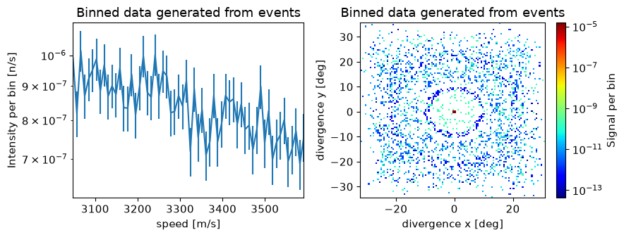
It is also possible to produce a McStasDataBinned dataset from a McStasDataEvent dataset by binning along one or two chosen dimensions using make_1d and make_2d. It supports all the same variables as above. For each method it is possible to choose how many bins should be used with the n_bins keyword argument.

speed_1d = events.make_1d("speed", n_bins=60)
divergence_2d = events.make_2d("dx", "dy", n_bins=[120, 120])

print(speed_1d)
print(divergence_2d)

McStasData: events type: 1D  I:4.9753504777625016e-05 E:5.021231142980946e-07 N:12442
McStasData: events type: 2D  I:4.975350477762497e-05 E:5.02123114298095e-07 N:12442.0

Plotting

McStasData objects contain information on how the data should be plotted, including for example if it should be on a logarithmic axis. This information is contained in the plot_options attribute of a McStasData object. The plotting are described in more detail on the plotting page.

PSD.plot_options

plot_options log: False
 colormap: jet
 show_colorbar: True
 cut_min: 0
 cut_max: 1
 x_limit_multiplier: 1
 y_limit_multiplier: 1

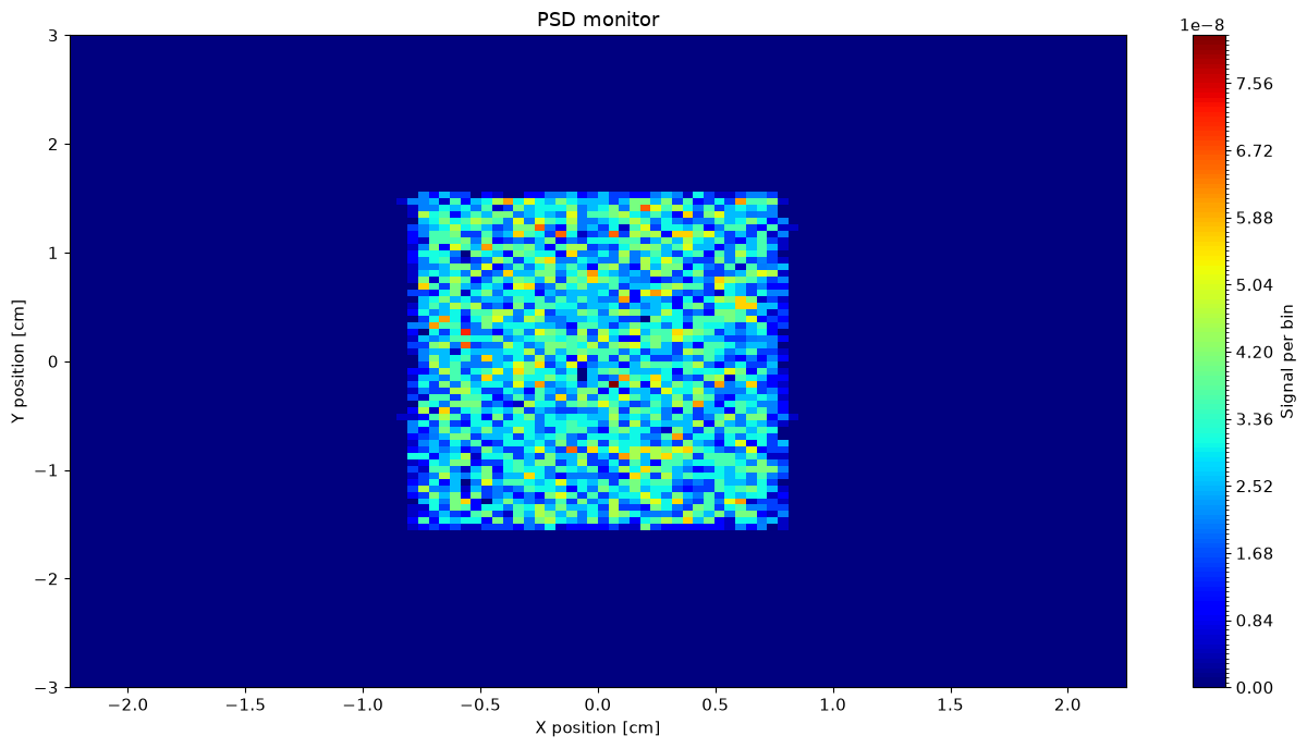
McStasScript can plot a McStasData object directly using for example make_plot.

ms.make_plot(PSD)

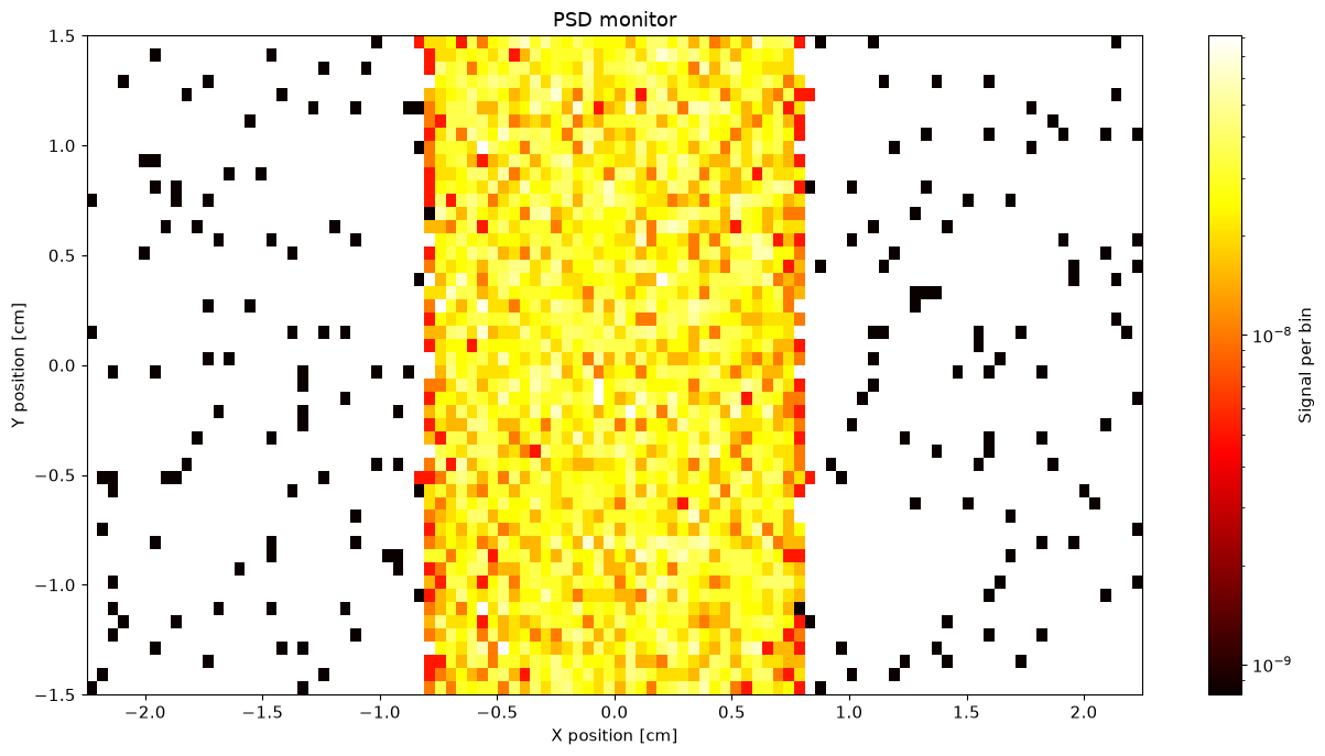
The plot_options can be updated with set_plot_options that takes keyword arguments.

PSD.set_plot_options(log=True, top_lim=1.5, bottom_lim=-1.5, colormap="hot", orders_of_mag=2)
ms.make_plot(PSD)

The set_plot_options takes the following keyword arguments. Some will only apply for 2D data, for example orders_of_mag.

Keyword argument	Type	Default	Description
log	bool	False	Logarithmic axis for y in 1D or z in 2D
orders_of_mag	float	300	Maximum orders of magnitude to plot in 2D
colormap	str	“jet”	Matplotlib colormap to use
show_colorbar	bool	True	Show the colorbar
x_axis_multiplier	float	1	Multiplier for x axis data
y_axis_multiplier	float	1	Multiplier for y axis data
cut_min	float	0	Unitless lower limit normalized to data range
cut_max	float	1	Unitless upper limit normalized to data range
left_lim	float		Lower limit to plot range of x axis
right_lim	float		Upper limit to plot range of x axis
bottom_lim	float		Lower limit to plot range of y axis
top_lim	float		Upper limit to plot range of y axis

McStasDataBinned generated from Event files can be plotted in the same manner.

ms.make_sub_plot([speed_1d, divergence_2d], log=True)