Plotting#

McStasScript includes a plotting module meant for plotting McStasScript data objects.

Example instrument#

First an example instrument is constructed to provide some data for plotting examples.

Hide code cell source

import mcstasscript as ms

instrument = ms.McStas_instr("data_example")

source = instrument.add_component("source", "Source_simple")
source.set_parameters(xwidth=0.05, yheight=0.03, dlambda=0.02,
                      dist=5, focus_xw=0.015, focus_yh=0.03)
source.lambda0 = instrument.add_parameter("wavelength", value=2.0)

sample = instrument.add_component("sample", "PowderN")
sample.set_parameters(radius=source.focus_xw, yheight=0.8*source.focus_yh,
                      reflections='"Na2Ca3Al2F14.laz"')
sample.set_AT(source.dist, RELATIVE=source)

banana = instrument.add_component("banana", "Monitor_nD", RELATIVE=sample)
banana.set_parameters(xwidth=1.5, yheight=0.4, restore_neutron=1, filename='"banana.dat"')
banana.options = '"theta limits=[5 175] bins=250, banana"'

mon = instrument.add_component("PSD", "PSD_monitor")
mon.set_AT(0.1, RELATIVE=sample)
mon.set_parameters(nx=100, ny=100, filename='"psd.dat"',
                   xwidth=5*sample.radius, yheight=2*sample.yheight, restore_neutron=1)

Performing the simulation#

Here the simulation is performed to provide the example data.

instrument.settings(ncount=1E6, output_path="plotting_example")
instrument.set_parameters(wavelength=1.5)
data = instrument.backengine()

Hide code cell output

INFO: Using directory: "/home/runner/work/McStasScript/McStasScript/docs/source/user_guide/plotting_example"
INFO: Regenerating c-file: data_example.c
CFLAGS= @NCRYSTALFLAGS@
          
WARNING:
 The parameter format of sample is initialized 
 using a static {,,,} vector.
  -> Such static vectors support literal numbers ONLY.
  -> Any vector use of variables or defines must happen via a 
     DECLARE/INITIALIZE pointer.


-----------------------------------------------------------

Generating single GPU kernel or single CPU section layout: 

-----------------------------------------------------------

Generating GPU/CPU -DFUNNEL layout:

-----------------------------------------------------------
INFO: Recompiling: ./data_example.out
lto-wrapper: warning: using serial compilation of 2 LTRANS jobs
lto-wrapper: note: see the '-flto' option documentation for more information
/home/runner/micromamba/envs/mcstasscript-docs/bin/x86_64-conda-linux-gnu-ld: /tmp/ccT62Abd.ltrans1.ltrans.o: in function `read_line_data.constprop.0':
/home/runner/work/McStasScript/McStasScript/docs/source/user_guide/./data_example.c:10259:(.text.read_line_data.constprop.0+0xea): warning: the use of `tmpnam' is dangerous, better use `mkstemp'
INFO: ===
Opening input file '/home/runner/micromamba/envs/mcstasscript-docs/share/mcstas/resources/data/Na2Ca3Al2F14.laz' (Table_Read_Offset)
Table from file 'Na2Ca3Al2F14.laz' (block 1) is 841 x 18 (x=1:20), constant step. interpolation: linear
  '# TITLE *-Na2Ca3Al2F14-[I213] Courbion, G.;Ferey, G.[1988] Standard NAC cal ...'
PowderN: sample: Reading 841 rows from Na2Ca3Al2F14.laz
PowderN: sample: Read 841 reflections from file 'Na2Ca3Al2F14.laz'
PowderN: sample: Vc=1079.1 [Angs] sigma_abs=11.7856 [barn] sigma_inc=13.6704 [barn] reflections=Na2Ca3Al2F14.laz
*** TRACE end *** 
Detector: banana_I=3.19138e-07 banana_ERR=1.95914e-09 banana_N=85837 "banana.dat"
Detector: PSD_I=7.21841e-06 PSD_ERR=1.85583e-08 PSD_N=284453 "psd.dat"
PowderN: sample: Info: you may highly improve the computation efficiency by using
    SPLIT 263 COMPONENT sample=PowderN(...)
  in the instrument description data_example.instr.
INFO: Placing instr file copy data_example.instr in dataset /home/runner/work/McStasScript/McStasScript/docs/source/user_guide/plotting_example
INFO: Placing generated c-code copy data_example.c in dataset /home/runner/work/McStasScript/McStasScript/docs/source/user_guide/plotting_example
print(data)
[
McStasData: banana type: 1D  I:3.19138e-07 E:1.95914e-09 N:85837.0, 
McStasData: PSD type: 2D  I:7.21841e-06 E:1.85583e-08 N:284453.0]

make_plot and make_sub_plot#

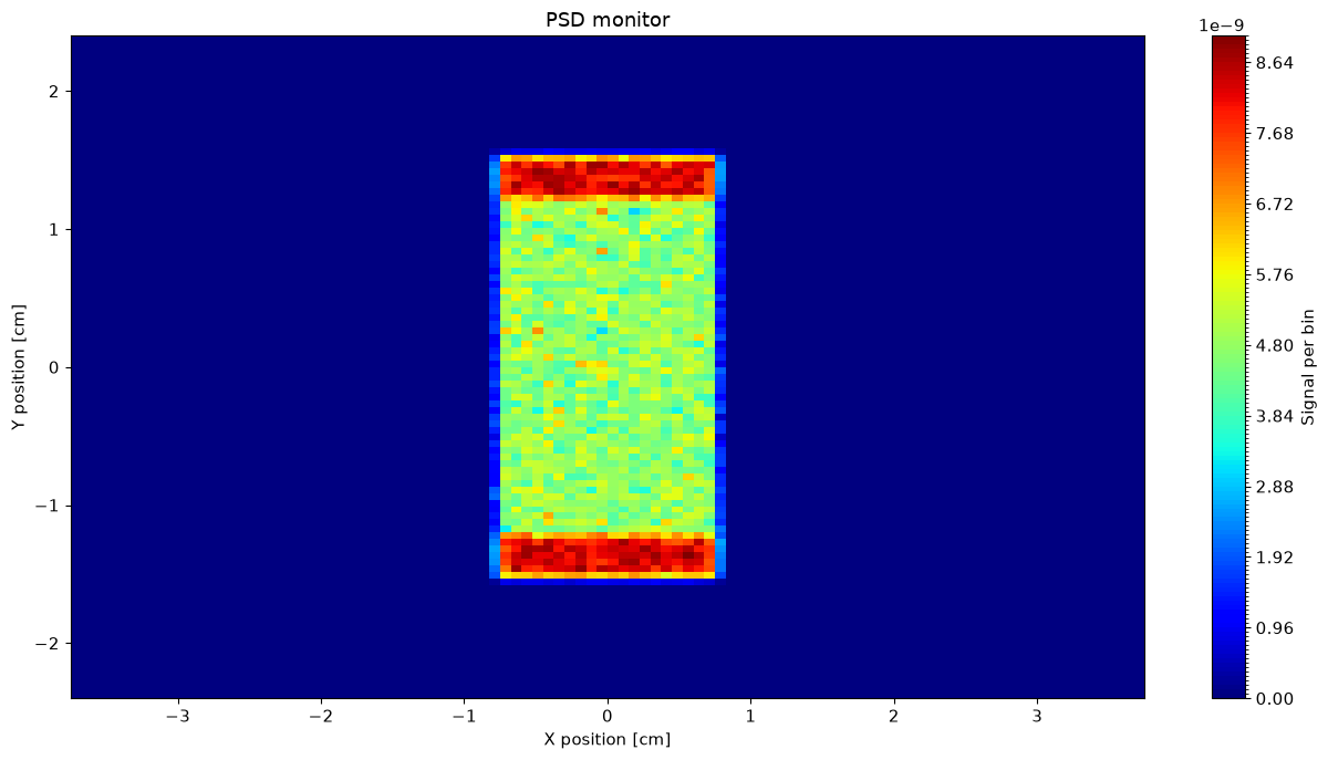
The first available plotter is make_plot, it makes a single figure for each McStasData set given in the input.

ms.make_plot(data)
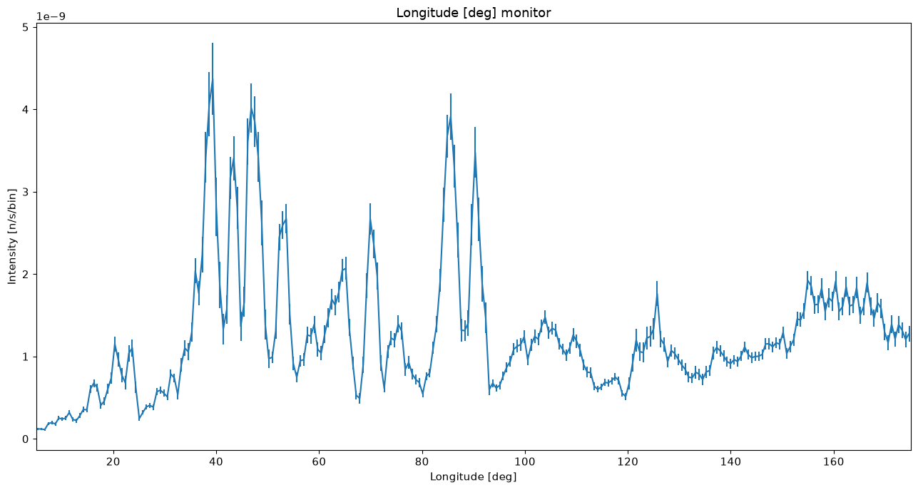
../_images/e1ff1617d72bbadcdeaf9d48eb23dd12f0f9cba72b93fdba09b0c2149b049089.png ../_images/5f852d466ace345a95bbd9a5f94382465d114448ccc21936ba6978049c60fda1.png

The second available plotter is make_sub_plot, it makes a single figure that includes plot of all given McStasData as subplots. This works best with between 1 and 9 monitors, as more tend to become difficult to read.

ms.make_sub_plot(data)
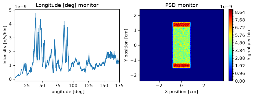
../_images/cff61b4879f7d4d731c5e07e6c7110516fea9c97ce9447c478b9b8a7e3b09bdd.png

Customizing plots#

As described in the data section of the documentation, the McStasData objects contain preferences on how they should be plotted. The same keywords can however be given to the plotters to override these preferences. When plotting a list of McStasData objects, a list can be given for each keyword.

ms.make_sub_plot(data, log=[False, True], fontsize=15)
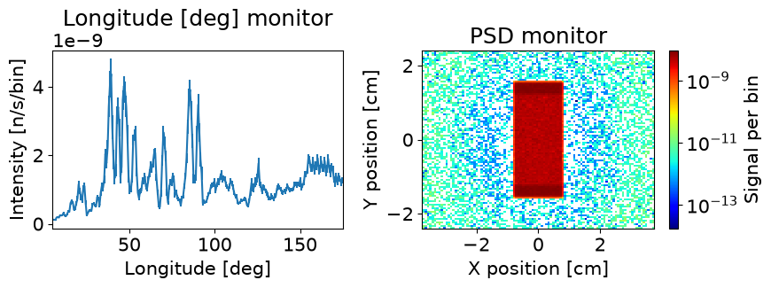
../_images/8b55997718776ad3653a244a68c55352763b4ae2d58eb2482010a5f8792b893e.png

Available keywords#

The keywords available to customize plotting are the same as can be set for plot_options in McStasData. There are however a few additional keywords for controlling figure size and fontsize.

Keyword argument

Type

Default

Description

figsize

tuple

(13, 7)

Tuple describing figure size

fontsize

int

11

Fontsize to use in plotting

log

bool

False

Logarithmic axis for y in 1D or z in 2D

orders_of_mag

float

300

Maximum orders of magnitude to plot in 2D

colormap

str

“jet”

Matplotlib colormap to use

show_colorbar

bool

True

Show the colorbar

x_axis_multiplier

float

1

Multiplier for x axis data

y_axis_multiplier

float

1

Multiplier for y axis data

cut_min

float

0

Unitless lower limit normalized to data range

cut_max

float

1

Unitless upper limit normalized to data range

left_lim

float

Lower limit to plot range of x axis

right_lim

float

Upper limit to plot range of x axis

bottom_lim

float

Lower limit to plot range of y axis

top_lim

float

Upper limit to plot range of y axis